Understanding Probability Flow ODE: Converting SDEs into Deterministic Sampling¶

1. Introduction¶

Score-based generative models (SBMs) and diffusion models rely on stochastic differential equations (SDEs) to model data distributions. However, while SDEs introduce randomness in sample trajectories, they can be converted into an equivalent ordinary differential equation (ODE) that retains the same probability density evolution. This ODE, known as the Probability Flow ODE , enables deterministic sampling while preserving the learned data distribution. This post will:

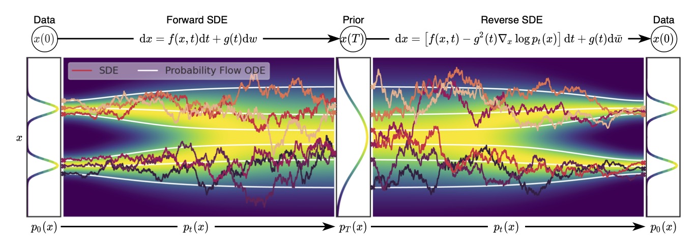
Explain how SDE-based models generate samples
Derive Probability Flow ODE from Fokker-Planck theory
Provide an intuitive understanding of why this works
Give a Python implementation for deterministic sampling

2. What is an SDE-Based Generative Model?¶

A stochastic differential equation (SDE) is used to describe how data evolves over time:

\[ dx = f(x, t) dt + g(t) dW \]

where:

$f(x, t)$ is the drift term (deterministic evolution).
$g(t) dW$ is the diffusion term (random noise from a Wiener process $dW$).
$p_t(x)$ is the time-dependent probability density of $x_t$. Since SDEs include random noise , different samples follow different trajectories even if they start at the same initial condition.

3. The Fokker-Planck Equation¶

The Key to Probability Density EvolutionAlthough each sample follows a random trajectory , the probability density function $p_t(x)$ follows a deterministic evolution governed by the Fokker-Planck equation (FPE) : $$ \frac{\partial p_t(x)}{\partial t} = -\nabla \cdot (f(x, t) p_t(x)) + \frac{1}{2} g^2(t) \nabla^2 p_t(x) $$

The first term $-\nabla \cdot (f(x, t) p_t(x))$ describes the effect of the drift term $f(x, t)$ on the probability density.
The second term $\frac{1}{2} g^2(t) \nabla^2 p_t(x)$ captures how diffusion smooths out the density over time. Even though each particle moves randomly, the overall probability distribution $p_t(x)$ evolves in a deterministic manner.

4. How Can We Convert an SDE into an ODE?¶

Since the probability density $p_t(x)$ follows a deterministic equation (FPE), there should exist a corresponding deterministic process that moves samples in a way that preserves the same $p_t(x)$.

This motivates the idea of a Probability Flow ODE :

\[ dx = v(x, t) dt \]

where $v(x, t)$ is a velocity field ensuring that the samples evolve according to the same probability density as the SDE, which is

\[ dx = \left[ f(x, t) - \frac{1}{2} g^2(t) s_t(x) \right] dt \]

where $s_t(x) = \nabla_x \log p_t(x)$ is the score function (gradient of the log density).

Proof: Convert SDE to Probability Flow ODE

Using the continuity equation from fluid mechanics, the deterministic probability flow should satisfy:

\[ \frac{\partial p_t(x)}{\partial t} = -\nabla \cdot (v(x, t) p_t(x)) \]

For this to be equivalent to the Fokker-Planck equation , we set:

\[ -\nabla \cdot (v(x, t) p_t(x)) = -\nabla \cdot (f(x, t) p_t(x)) + \frac{1}{2} g^2(t) \nabla^2 p_t(x) \]

Rearranging:

\[ v(x, t) p_t(x) = f(x, t) p_t(x) - \frac{1}{2} g^2(t) \nabla p_t(x) \]

Dividing by $p_t(x)$ (assuming $p_t(x) > 0$):

\[ v(x, t) = f(x, t) - \frac{1}{2} g^2(t) \frac{\nabla p_t(x)}{p_t(x)} \]

Since the score function is:

\[ s_t(x) = \nabla_x \log p_t(x) = \frac{\nabla_x p_t(x)}{p_t(x)} \]

we obtain the Probability Flow ODE :

\[ dx = \left[ f(x, t) - \frac{1}{2} g^2(t) s_t(x) \right] dt \]

Thus, we have converted the original SDE into an equivalent deterministic ODE that preserves the same probability density evolution!

5. Intuition: Why Does This Work?¶

SDE = Particles move randomly, but their overall density evolves deterministically.
ODE = Particles move deterministically in a way that ensures the density evolves the same way.

Thus, we can replace SDE sampling with Probability Flow ODE sampling without changing the generated distribution!

6. Implementing Probability Flow ODE Sampling¶

We can implement Probability Flow ODE sampling using an ODE solver like torchdiffeq.odeint:

import torch
from torchdiffeq import odeint

def probability_flow_ode(x, t, score_model):
    score = score_model(x, t)  # Compute score function s_t(x)
    drift = f(x, t) - 0.5 * g(t)**2 * score
    return drift

# Solve the ODE to generate samples
x_generated = odeint(probability_flow_ode, x_init, t_space)

Key difference from SDE sampling :
No randomness → Every run gives identical outputs.
Faster sampling → Fewer steps needed than stochastic diffusion.

7. Existence Condition and Uniqueness Condition¶

Existence Conditions

For $v(x, t)$ to exist , the following conditions must hold:

Condition	Explanation
$p_t(x)$ is continuously differentiable ($p_t(x) \in C^1$)	Ensures that $\nabla_x p_t(x)$ and $\nabla_x \log p_t(x)$ are well-defined.
$p_t(x) > 0$ for all $x$	Avoids division by zero in the score function $s_t(x) = \nabla_x \log p_t(x)$.
Drift term $f(x, t)$ is well-defined	Ensures the continuity equation has a meaningful solution.
$p_t(x)$ evolves deterministically under Fokker-Planck equation	The probability density function should not be singular.
$g(t) > 0$ (Non-degenerate diffusion)	If $g(t) = 0$, then the SDE is already deterministic and trivially satisfies an ODE.

Uniqueness Conditions

Condition	Explanation
$p_t(x)$ is log-concave ($\nabla^2 \log p_t(x) \preceq 0$)	Ensures the score function $s_t(x) = \nabla_x \log p_t(x)$ is unique and stable.
No divergence-free component in $v(x, t)$	If an alternative field $v'(x,t)=v(x,t)+v_{div-free}(x,t)$ exists, $v(x, t)$ is not unique.
$p_t(x)$ is strictly positive and smooth	Avoids singularities and undefined score function regions.
Drift term $f(x, t)$ is uniquely defined	Ensures a single solution to the continuity equation.

8. Experiment¶

8.1 Target Distribution¶

The Funnel distribution is defined as follows:

$ v \sim \mathcal{N}(0, 3^2) $
$ x \mid v \sim \mathcal{N}\bigl(0, \exp(v)\bigr) $

Thus, the joint density is given by:

\[ p(x,v) = \frac{1}{3\sqrt{2\pi}} \exp\left(-\frac{v^2}{18}\right) \cdot \frac{1}{\sqrt{2\pi\,\exp(v)}} \exp\left(-\frac{x^2}{2\exp(v)}\right) \]

import torch
import matplotlib.pyplot as plt
import seaborn as sns
from sklearn.datasets import make_swiss_roll
def sample_funnel_data(num_samples=10000):
    """
    从简化 2D funnel 分布中采样:
    z ~ N(0, 1)
    x ~ N(0, exp(z))
    返回 shape: (num_samples, 2)
    """
    z = torch.randn(num_samples)*0.8
    x = torch.randn(num_samples) * torch.exp(z )/5  # exp(z/2) 的方差 = exp(z)
    data = torch.stack([x,z], dim=1)  # shape [num_samples, 2]
    return data

8.2 sampling formula¶

Below are the expressions for the original distribution, the Langevin (diffusion) process, the DDPM reverse diffusion SDE, and the corresponding probability flow ODE for DDPM sampling.

8.2.1 Langevin Diffusion Expression¶

In overdamped Langevin dynamics, the update rule for a state $ z = (x,v) $ is:

\[ z_{t+1} = z_t + \epsilon\,\nabla_z \log p(z_t) + \sqrt{2\epsilon}\,\xi_t,\quad \xi_t \sim \mathcal{N}(0, I) \]

This iterative update gradually moves samples toward the target distribution $ p(x,v) $.

8.2.2 DDPM Reverse Diffusion SDE¶

For a variance-preserving (VP) forward SDE defined as

\[ dx = -\frac{1}{2}\beta(t)x\,dt + \sqrt{\beta(t)}\,dW_t, \]

the reverse-time SDE used for sampling (starting from pure Gaussian noise at $ t=1 $) is:

\[ dx = \left[-\frac{1}{2}\beta(t)x - \beta(t)\nabla_x\log p_t(x)\right]\,dt + \sqrt{\beta(t)}\,d\bar{W}_t. \]

Here, $ \nabla_x\log p_t(x) $ is the score function at time $ t $.

8.2.3 DDPM Probability Flow ODE¶

The deterministic probability flow ODE corresponding to the DDPM SDE is given by:

\[ dx = \left[-\frac{1}{2}\beta(t)x - \frac{1}{2}\beta(t)\nabla_x\log p_t(x)\right]\,dt. \]

Solving this ODE from $ t=1 $ (Gaussian noise) to $ t=0 $ yields samples that follow the target distribution.

These expressions form the basis for diffusion-based generative modeling—from the formulation of the target distribution to sampling via both stochastic reverse diffusion and its deterministic ODE counterpart.

8.3 Results on different sampling methods¶

8.3.1 VP-SDE¶

8.3.1.1 Sampling Annimation¶


Langervin Dynamic	VP-SDE	VP-SDE FLow ODE	DDPM

8.3.1.2 Codes¶

ddpmVP-SDE trainingVP-SDE samplingVP-SDE FLOW ODE samplingLangervin Dynamic samplingmake annimation

ddpm training and sampling
import torch
import torch.nn as nn
class DiffusionBlock(nn.Module):
    def **init**(self, nunits):
        super(DiffusionBlock, self).**init**()
        self.linear = nn.Linear(nunits, nunits)
    def forward(self, x: torch.Tensor):
        x = self.linear(x)
        x = nn.functional.relu(x)
        return x
class DiffusionModel(nn.Module):
    def **init**(self, nfeatures: int, nblocks: int = 2, nunits: int = 64):
        super(DiffusionModel, self).**init**()
        self.inblock = nn.Linear(nfeatures+1, nunits)
        self.midblocks = nn.ModuleList([DiffusionBlock(nunits) for _ in range(nblocks)])
        self.outblock = nn.Linear(nunits, nfeatures)
    def forward(self, x: torch.Tensor, t: torch.Tensor) -> torch.Tensor:
        val = torch.hstack([x, t])  # Add t to inputs
        val = self.inblock(val)
        for midblock in self.midblocks:
            val = midblock(val)
        val = self.outblock(val)
        return val
model = DiffusionModel(nfeatures=2, nblocks=4)
device = "cuda"
model = model.to(device)
import torch.optim as optim
nepochs = 100
batch_size = 2048
loss_fn = nn.MSELoss()
optimizer = optim.Adam(model.parameters(), lr=0.001)
scheduler = optim.lr_scheduler.LinearLR(optimizer, start_factor=1.0, end_factor=0.01, total_iters=nepochs)
for epoch in range(nepochs):
    epoch_loss = steps = 0
    for i in range(0, len(X), batch_size):
        Xbatch = X[i:i+batch_size]
        timesteps = torch.randint(0, diffusion_steps, size=[len(Xbatch), 1])
        noised, eps = noise(Xbatch, timesteps)
        predicted_noise = model(noised.to(device), timesteps.to(device))
        loss = loss_fn(predicted_noise, eps.to(device))
        optimizer.zero_grad()
        loss.backward()
        optimizer.step()
        epoch_loss += loss
        steps += 1
    print(f"Epoch {epoch} loss = {epoch_loss / steps}")
def sample_ddpm(model, nsamples, nfeatures):
    """Sampler following the Denoising Diffusion Probabilistic Models method by Ho et al (Algorithm 2)"""
    with torch.no_grad():
        x = torch.randn(size=(nsamples, nfeatures)).to(device)
        xt = [x]
        for t in range(diffusion_steps-1, 0, -1):
            predicted_noise = model(x, torch.full([nsamples, 1], t).to(device))
            # See DDPM paper between equations 11 and 12
            x = 1 / (alphas[t] ** 0.5) * (x - (1 - alphas[t]) / ((1-baralphas[t]) ** 0.5) * predicted_noise)
            if t > 1:
                # See DDPM paper section 3.2.
                # Choosing the variance through beta_t is optimal for x_0 a normal distribution
                variance = betas[t]
                std = variance ** (0.5)
                x += std * torch.randn(size=(nsamples, nfeatures)).to(device)
            xt += [x]
        return x, xt

VP-SDE training
import torch
import torch.nn as nn
import torch.optim as optim
import matplotlib.pyplot as plt
import seaborn as sns
import torch
import torch.nn as nn
import torch.optim as optim
from torch.utils.data import DataLoader, TensorDataset
# Function to generate funnel data
def sample_funnel_data(num_samples=10000):
    z = torch.randn(num_samples) * 0.8
    x = torch.randn(num_samples) * torch.exp(z) / 5
    return torch.stack([x, z], dim=1)
class ScoreModel(nn.Module):
    def __init__(self, hidden_dims=[128, 256, 128], embed_dim=64):
        super().__init__()
        # 时间嵌入层
        self.embed = nn.Sequential(
            nn.Linear(1, embed_dim),
            nn.SiLU(),
            nn.Linear(embed_dim, embed_dim)
        )
        # 主干网络
        self.net = nn.ModuleList()
        input_dim = 2  # 输入维度
        for h_dim in hidden_dims:
            self.net.append(nn.Sequential(
                nn.Linear(input_dim + embed_dim, h_dim),
                nn.SiLU()))
            input_dim = h_dim
        self.out = nn.Linear(input_dim, 2)  # 输出噪声预测

    def forward(self, x, t):
        t_embed = self.embed(t)
        for layer in self.net:
            x = layer(torch.cat([x, t_embed], dim=1))
        return self.out(x)
# 训练参数
beta_min, beta_max = 0.1, 20.0
device = torch.device('cuda' if torch.cuda.is_available() else 'cpu')
# device ='cpu'
model = ScoreModel().to(device)
optimizer = optim.Adam(model.parameters(), lr=3e-4)
# 准备数据
data = sample_funnel_data(100000)
dataset = TensorDataset(data)
dataloader = DataLoader(dataset, batch_size=512, shuffle=True)
from tqdm import tqdm
# 训练循环
for epoch in tqdm(range(200)):
    total_loss = 0.0
    for batch, in dataloader:
        x0 = batch.to(device)
        batch_size = x0.size(0)
        # 采样时间和噪声
        t = torch.rand(batch_size, 1, device=device)
        epsilon = torch.randn_like(x0, device=device)
        # 计算 α(t) 和 σ(t)
        integral = beta_min * t + 0.5 * (beta_max - beta_min) * t**2
        alpha = torch.exp(-integral)
        sigma = torch.sqrt(1.0 - alpha)
        # 扰动数据
        x_t = torch.sqrt(alpha) * x0 + torch.sqrt(1.0 - alpha) * epsilon
        # 预测噪声
        score_pred = model(x_t, t)
        # 计算加权损失
        # beta_t = beta_min + (beta_max - beta_min) * t
        # print((1-alpha))
        loss = torch.mean( (score_pred - epsilon)**2) # predict is the score
        # 反向传播
        optimizer.zero_grad()
        loss.backward()
        optimizer.step()
        total_loss += loss.item() * batch_size
    if (epoch+1) % 20 == 0:
        print(f"Epoch {epoch+1}, Loss: {total_loss/len(data):.5f}")

VP SDE sampling

import torch
import numpy as np
import math
import matplotlib.pyplot as plt
def vp_sde_sample(model,x_T, timesteps, beta_min=0.1, beta_max=20.0, save_trajectory=True):
    """
    Implements the reverse sampling process for VP-SDE using Euler-Maruyama method.
    Args:
        x_T: Final noisy sample (torch.Tensor) of shape (N, D)
        timesteps: Number of diffusion steps (int)
        beta_min: Minimum beta value (float)
        beta_max: Maximum beta value (float)
        save_trajectory: Whether to save and return the sampling trajectory (bool)
    Returns:
        x_0: Recovered data sample (torch.Tensor)
        trajectory: List of intermediate states (if save_trajectory=True)
    """
    dt = 1.0 / timesteps  # Time step for numerical integration
    x_t = x_T.clone()
    trajectory = [x_t.clone().cpu().numpy()] if save_trajectory else None
    model  = model.eval()
    for t_index in reversed(range(1,timesteps)):
        t = t_index * dt
        print("t",t, end="\r")
        # 计算 α(t) 和 σ(t)
        integral = beta_min * t + 0.5 * (beta_max - beta_min) * t**2
        integral = torch.Tensor([integral])
        alpha = torch.exp(-integral)
        beta_t = beta_min +  (beta_max - beta_min) * t
        beta_t = torch.Tensor([beta_t])
        with torch.no_grad():
            t_input = torch.Tensor([t]*len(x_t)).to(device).unsqueeze(-1)
            # print('x_t',x_t.shape, t_input.shape)
            noise_pred = model(x_t.to(device),t_input)
            if  not torch.isfinite(noise_pred).all():
                print('score_function got nan',score_function,t_index)
                raise
            score_function = - noise_pred.cpu() / torch.sqrt(1-alpha)
        s_theta  = score_function.cpu()
        # Reverse SDE Euler-Maruyama step
        x_t = x_t +1/2 * beta_t *( x_t +2* s_theta)* dt # dritf term
        x_t += torch.sqrt(beta_t) * torch.randn_like(x_t) * math.sqrt(dt) # diffusion term
        if  not torch.isfinite(x_t).all():
            print("xt got infinite", t_index, x_t[:2],torch.sqrt(1-alpha))
        if save_trajectory:
            trajectory.append(x_t.clone().cpu().numpy())
    return x_t, trajectory if save_trajectory else None
# Set parameters
timesteps = 1500
num_samples = 20000
dim = 2  # 2D distribution for visualization
x_T = torch.randn(num_samples, dim)  # Sample from Gaussian prior (standard normal)
# Perform VP-SDE sampling
x_0, trajectory = vp_sde_sample(model, x_T, timesteps)
# Convert trajectory to numpy for plotting
trajectory_np = np.array(trajectory)  # Shape: (timesteps, num_samples, dim)
# Plot final distribution shape
plt.figure(figsize=(6, 6))
plt.scatter(x_0[:, 0].numpy(), x_0[:, 1].numpy(), alpha=0.5, s=10)
plt.title("Final Sampled Distribution from VP-SDE")
plt.xlabel("X-axis")
plt.ylabel("Y-axis")
plt.axis("equal")
plt.show()

VP-SDE FLOW ODE sampling

import torch
import numpy as np
import math
import matplotlib.pyplot as plt
def vp_ode_sample(model,x_T, timesteps, beta_min=0.1, beta_max=20.0, save_trajectory=True):
    """
    Implements the reverse sampling process for VP-SDE using Euler-Maruyama method.
    Args:
        x_T: Final noisy sample (torch.Tensor) of shape (N, D)
        timesteps: Number of diffusion steps (int)
        beta_min: Minimum beta value (float)
        beta_max: Maximum beta value (float)
        save_trajectory: Whether to save and return the sampling trajectory (bool)
    Returns:
        x_0: Recovered data sample (torch.Tensor)
        trajectory: List of intermediate states (if save_trajectory=True)
    """
    dt = 1.0 / timesteps  # Time step for numerical integration
    x_t = x_T.clone()
    trajectory = [x_t.clone().cpu().numpy()] if save_trajectory else None
    model  = model.eval()
    for t_index in reversed(range(1,timesteps)):
        t = t_index *dt
        print("t",t, end="\r")
        # 计算 α(t) 和 σ(t)
        integral = beta_min* t + 0.5 *(beta_max - beta_min)* t**2
        integral = torch.Tensor([integral])
        alpha = torch.exp(-integral)
        beta_t = beta_min +  (beta_max - beta_min) *t
        beta_t = torch.Tensor([beta_t])
        with torch.no_grad():
            t_input = torch.Tensor([t]*len(x_t)).to(device).unsqueeze(-1)
            # print('x_t',x_t.shape, t_input.shape)
            noise_pred = model(x_t.to(device),t_input)
            if  not torch.isfinite(noise_pred).all():
                print('score_function got nan',score_function,t_index)
                raise
            score_function = - noise_pred.cpu() / torch.sqrt(1-alpha)
        s_theta  = score_function.cpu()
        # Reverse SDE Euler-Maruyama step
        # x_t = x_t +1/2 * beta_t *( x_t +2* s_theta)* dt # dritf term
        # x_t += torch.sqrt(beta_t)* torch.randn_like(x_t) *math.sqrt(dt) # diffusion term
        x_t = x_t +1/2* beta_t *( x_t + s_theta)* dt
        if  not torch.isfinite(x_t).all():
            print("xt got infinite", t_index, x_t[:2],torch.sqrt(1-alpha))
        if save_trajectory:
            trajectory.append(x_t.clone().cpu().numpy())
    return x_t, trajectory if save_trajectory else None
# Set parameters
timesteps = 1500
num_samples = 20000
dim = 2  # 2D distribution for visualization
x_T = torch.randn(num_samples, dim)  # Sample from Gaussian prior (standard normal)
# Perform VP-SDE sampling
x_0, trajectory = vp_ode_sample(model, x_T, timesteps)
# Convert trajectory to numpy for plotting
trajectory_np = np.array(trajectory)  # Shape: (timesteps, num_samples, dim)
# Plot final distribution shape
plt.figure(figsize=(6, 6))
plt.scatter(x_0[:, 0].numpy(), x_0[:, 1].numpy(), alpha=0.5, s=10)
plt.title("Final Sampled Distribution from VP-SDE")
plt.xlabel("X-axis")
plt.ylabel("Y-axis")
plt.axis("equal")
plt.show()

Langervin Dynamic sampling
    import torch
    import matplotlib.pyplot as plt
    def funnel_score(x, z):
        """Compute the score function (gradient of log-density) of the funnel distribution."""
        score_x = -x / torch.exp(z)
        score_z = -z + 0.5 * x**2 * torch.exp(-z)
        return torch.stack([score_x, score_z], dim=1)
    def langevin_sampling_funnel(num_samples=10000, lr=0.001, num_steps=1500, noise_scale=0.001):
        """Sample from the funnel distribution using Langevin dynamics."""
        # Initialize samples from a normal distribution
        samples = torch.randn(num_samples, 2)
        trajectory = [samples.clone()]  # Store trajectory
        for _ in range(num_steps):
            x, z = samples[:, 0], samples[:, 1]
            score = funnel_score(x, z)
            samples = samples + lr * score + math.sqrt(2*noise_scale) * torch.randn_like(samples)
            trajectory.append(samples.clone())  # Store trajectory step
        return samples, trajectory
    # Sample using Langevin dynamics
    samples, trajectory = langevin_sampling_funnel()
    # Convert trajectory to numpy for visualization
    trajectory_np = [step.numpy() for step in trajectory]
    # Plot final distribution
    plt.figure(figsize=(6, 6))
    plt.scatter(samples[:, 0], samples[:, 1], alpha=0.5, s=0.1)
    plt.title("Final Sampled Distribution from VP-SDE")
    plt.xlabel("X-axis")
    plt.ylabel("Y-axis")
    plt.axis("equal")
    plt.show()

from matplotlib.animation import FuncAnimation, PillowWriter
def make_animation(trajectory, filename="sampling.gif"):
    """
    Given a list of [N x 2] arrays (trajectory), create and save an animation.
    """
    trajectory = [x.cpu() for x in trajectory]
    fig, ax = plt.subplots(figsize=(5, 5))
    scat = ax.scatter(trajectory[0][:, 0], trajectory[0][:, 1], alpha=0.5, color='red',s=0.2)
    ax.set_xlim(-6, 6)
    ax.set_ylim(-6, 6)
    ax.axis("off")
    ax.set_aspect('equal')
    time_text = ax.text(0.02, 0.02, '', transform=ax.transAxes, fontsize=12)
    def update(frame):
        data = trajectory[frame]
        scat.set_offsets(data)
        time_text.set_text(f"Step {frame}/{len(trajectory)-1}")
        return scat, time_text
    ani = FuncAnimation(fig, update, frames=len(trajectory), interval=1)
    writer = PillowWriter(fps=40)
    ani.save(filename, writer=writer)
    plt.close()
...
make_animation(trajectory_np, filename=img_file)

8.3.2 VE-SDE¶

Let's experiment with VE-SDE. First, just recall the formulas to understand the dynamics:

Forward Process (SDE)

\[ dx = \sqrt{\frac{d[\sigma^2(t)]}{dt}} dw \]

Noise Schedule

\[ \sigma_t = \sigma_{\text{min}} \left(\frac{\sigma_{\text{max}}}{\sigma_{\text{min}}} \right)^t \]

Sampling from Noisy Distribution

\[ x_t = x_0 + \sigma_t \epsilon, \quad \epsilon \sim \mathcal{N}(0, I) \]

Reverse Process (SDE)

\[ dx = - \left(\frac{d[\sigma^2(t)]}{dt} \right) \nabla_x \log p_t(x) dt + \sqrt{\frac{d[\sigma^2(t)]}{dt}} dw \]

derivateve of $\sigma(t)$

\[ \frac{d \sigma^2(t)}{dt} = \sigma_{\text{min}}^2 \left(\frac{\sigma_{\text{max}}^2}{\sigma_{\text{min}}^2} \right)^t \log \left(\frac{\sigma_{\text{max}}^2}{\sigma_{\text{min}}^2} \right) \]

Flow ODE (Deterministic Approximation)

\[ dx = -\frac{1}{2}\left(\frac{d[\sigma^2(t)]}{dt} \right) \nabla_x \log p_t(x) dt \]

Reverse Sampling

\[ x_{t-1} = x_t + \left(\frac{d[\sigma^2(t)]}{dt} \right) s_{\theta}(x, t) dt \]

Score Function

\[ s_{\theta}(x, t) = -\frac{\epsilon}{\sigma_t} \]

Loss Function (Score Matching)

\[ \mathbb{E}_{t, x_0, \epsilon} \left[ \lambda_t \left\| s_{\theta}(x_t, t) + \frac{\epsilon}{\sigma_t} \right\|^2 \right] \]

8.3.2.1 Sampling Results¶

docs/images/ve_ode.gif


ve-sde	ve-sde flow ODE	DP-SDE flow ODE	DDPM

9. Conclusion¶

Every SDE can be converted into a Probability Flow ODE.
The deterministic ODE preserves the same probability density as the SDE.
Probability Flow ODE allows for efficient, repeatable sampling.
ODE solvers can be used instead of SDE solvers for generative modeling. By leveraging Probability Flow ODE, we gain a powerful tool for deterministic yet efficient sampling in deep generative models . 🚀

10. Further Reading¶

Song et al., "Score-Based Generative Modeling through Stochastic Differential Equations," NeurIPS 2021
Chen et al., "Neural ODEs," NeurIPS 2018
Fluid mechanics: Continuity equation and probability flow
"The Probability Flow ODE is Provably Fast" Authors: Sitan Chen, Sinho Chewi, Holden Lee, Yuanzhi Li, Jianfeng Lu, Adil Salim Summary: This paper provides the first polynomial-time convergence guarantees for the probability flow ODE implementation in score-based generative modeling. The authors develop novel techniques to study deterministic dynamics without contractivity. Link: arXiv:2305.11798
"Convergence Analysis of Probability Flow ODE for Score-based Generative Models" Authors: Daniel Zhengyu Huang, Jiaoyang Huang, Zhengjiang Lin Summary: This work studies the convergence properties of deterministic samplers based on probability flow ODEs, providing theoretical bounds on the total variation between the target and generated distributions. Link: arXiv:2404.09730 2. Practical Implementations and Tutorials:
"On the Probability Flow ODE of Langevin Dynamics" Author: Mingxuan Yi Summary: This blog post offers a numerical approach using PyTorch to simulate the probability flow ODE of Langevin dynamics, providing insights into practical implementation. Link: Mingxuan Yi's Blog
"Generative Modeling by Estimating Gradients of the Data Distribution" Author: Yang Song Summary: This post discusses learning score functions (gradients of log probability density functions) on noise-perturbed data distributions and generating samples with Langevin-type sampling. Link: Yang Song's Blog 3. Advanced Topics and Related Methods:
"An Introduction to Flow Matching" Authors: Cambridge Machine Learning Group Summary: This blog post introduces Flow Matching, a generative modeling paradigm combining aspects from Continuous Normalizing Flows and Diffusion Models, offering a unique perspective on generative modeling. Link: Cambridge MLG Blog
"Flow Matching: Matching Flows Instead of Scores" Author: Jakub M. Tomczak Summary: This article presents a different perspective on generative models with ODEs, discussing Continuous Normalizing Flows and Probability Flow ODEs. Link: Jakub M. Tomczak's Blog

Condition	Explanation
\(p_t(x)\) is continuously differentiable (\(p_t(x) \in C^1\))	Ensures that \(\nabla_x p_t(x)\) and \(\nabla_x \log p_t(x)\) are well-defined.
\(p_t(x) > 0\) for all \(x\)	Avoids division by zero in the score function \(s_t(x) = \nabla_x \log p_t(x)\).
Drift term \(f(x, t)\) is well-defined	Ensures the continuity equation has a meaningful solution.
\(p_t(x)\) evolves deterministically under Fokker-Planck equation	The probability density function should not be singular.
\(g(t) > 0\) (Non-degenerate diffusion)	If \(g(t) = 0\), then the SDE is already deterministic and trivially satisfies an ODE.

Condition	Explanation
\(p_t(x)\) is log-concave (\(\nabla^2 \log p_t(x) \preceq 0\))	Ensures the score function \(s_t(x) = \nabla_x \log p_t(x)\) is unique and stable.
No divergence-free component in \(v(x, t)\)	If an alternative field \(v'(x,t)=v(x,t)+v_{div-free}(x,t)\) exists, \(v(x, t)\) is not unique.
\(p_t(x)\) is strictly positive and smooth	Avoids singularities and undefined score function regions.
Drift term \(f(x, t)\) is uniquely defined	Ensures a single solution to the continuity equation.