Stochastic Differential Equation for DDPM

In this section, we will explore how Stochastic Differential Equations (SDEs) are connected to the denoising diffusion probabilistic model and the denoising score matching.

1. Forward Diffusion Process

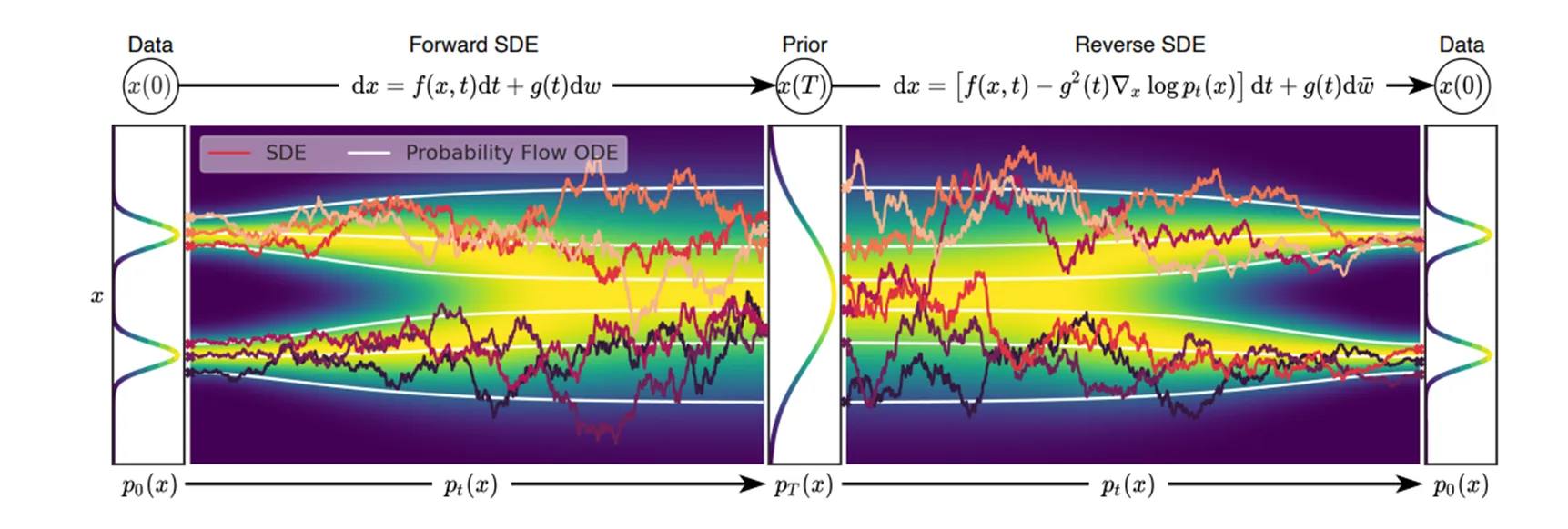
The forward diffusion process is described by a stochastic differential equation (SDE) that gradually adds noise to the data. The general form of this forward SDE is:

\[ \tag{1} dx \;=\; f(x,t)\,dt \;+\; g(t)\,dW_t \]

where:

• \(f(x,t)\) is the drift term that controls the deterministic evolution
• \(g(t)\) is the diffusion coefficient that modulates the noise intensity
• \(W_t\) represents a standard Wiener process (Brownian motion)
• \(p_t(x)\) denotes the probability density of the state \(x\) at time \(t\)

For simplicity, we assume \(g(t)\) depends only on time, not space, though it may vary throughout the diffusion process.

2. Reverse Diffusion Process

The reverse diffusion process describes how we can recover the original data distribution by reversing the noise addition process. For a system with probability density \(p_t(x)\) at time \(t\), the Fokker-Planck equation yields the following reverse SDE:

\[ \tag{2} dx \;=\; \bigl[f(x,t)\;-\;g(t)^2\,\nabla_x \log p_{t}(x)\bigr]\;dt \;+\; g(t)\,d\overline{W}_t \]

This equation has two key components:

1. A drift term \(f(x,t)\) from the forward process
2. A score-based correction term \(-g(t)^2\,\nabla_x \log p_{t}(x)\) that guides the system toward higher probability regions

In the following sections, we'll derive this backward diffusion equation and explain why it correctly describes the time-reversal of our forward process.

2.1 Fokker–Planck (Forward Kolmogorov) Equation

The density \(p_t(x)\) satisfies the Fokker–Planck (or forward‐Kolmogorov) PDE

\[\tag{3} \frac{\partial p_t(x)}{\partial t} \;=\; -\nabla\!\cdot\!\bigl[f(x,t)\,p_t(x)\bigr] \;+\; \frac{1}{2}\,g(t)^2\,\Delta p_t(x), \]

where \(\Delta\) is the Laplacian in \(x\).

note

In one dimension , the Laplacian simplifies to:

\[ \Delta p_t(x) = \frac{\partial^2 p_t(x)}{\partial x^2} \]

In higher dimensions , the Laplacian is given by:

\[ \Delta p_t(x) = \sum_{i=1}^{d} \frac{\partial^2 p_t(x)}{\partial x_i^2} \]

where \(d\) is the dimension of the space. Thus, in the context of the Fokker-Planck equation, the Laplacian term governs the diffusive spreading of the probability density due to the noise term \(g(t) dW_t\) in the associated SDE.

Importance of the Fokker-Planck Equation

The Fokker-Planck equation (also known as the forward Kolmogorov equation) is a fundamental equation that describes the temporal evolution of probability distributions in stochastic processes. Its significance spans multiple fields including physics, finance, biology, and chemistry. Here's why it's crucial:

1. Evolution of Probability Distributions The Fokker-Planck equation computes the probability distribution of a system described by Stochastic Differential Equations (SDEs) at different time points, rather than tracking individual sample paths. This provides a complete statistical description of the system's behavior. This represents a fundamental shift in how we model system evolution: - In deterministic systems, we use Ordinary Differential Equations (ODEs) to describe the evolution of states directly - In stochastic systems, we use the Fokker-Planck equation to describe how the Probability Density Function (PDF) of states evolves over time

2. Bridging SDEs and Probability Distributions While Stochastic Differential Equations (SDEs) typically simulate individual sample paths, the Fokker-Planck equation provides a more comprehensive view of the probability distribution evolution: - SDE 给出的是随机轨迹，而 Fokker-Planck 方程提供了整体统计特性。 - 通过求解 Fokker-Planck 方程，可以获得系统的稳态分布，甚至预测其长期行为。

3. 适用于多个科学领域 Fokker-Planck 方程在多个学科领域都具有广泛应用

• 统计物理与热力学
  • 描述布朗运动（粒子在流体中的扩散）。
  • 用于朗之万方程（Langevin equation）的概率描述，研究噪声对物理系统的影响。
  • 计算非平衡系统的稳态分布，例如电场中的带电粒子运动。
• 生物学与生态系统
  • 在种群动力学中，描述随机环境下的种群演化（如随机 Logistic 模型）。
  • 研究神经元放电中的随机效应（Fokker-Planck 形式的神经动力学模型）。
  • 研究蛋白质折叠和细胞信号传导中的分子噪声影响。
• 金融与经济学
  • 在金融数学中，Fokker-Planck 方程与Black-Scholes 方程（用于期权定价）密切相关。
  • 描述股票价格分布，建模市场中资产价格的演化。
  • 用于计算风险分布，分析投资组合的长期收益分布。
• 化学与分子动力学
  • 研究化学反应中的随机过程，如反应扩散系统。
  • 在分子动力学中，描述带噪声的粒子运动，如高分子扩散。

4. 计算稳态解与动态分布 - 在长时间极限下，Fokker-Planck 方程的解可能趋于稳态分布（平衡解），用于分析长期稳定性。 - 在短时间范围内，方程提供了时间演化信息，帮助研究系统的短期行为。

总结 Fokker-Planck 方程是随机动力系统的核心工具，能够在多种科学和工程领域中提供概率分布的详细描述。相比单纯使用 SDE 进行模拟，Fokker-Planck 方程提供了更深入的数学理解，特别是在稳态分析、分布演化以及随机系统长期行为预测方面具有重要意义。

✅ SDE 描述个体行为，是随机的。 ✅ FPE 描述总体概率分布，是确定的。 ✅ FPE 提供了更稳定的系统描述，可用于长期分析和稳态计算。

Now we prove that the reverse diffusion formula

2.2 Strategy Diffusion Derivation

We want an SDE whose sample paths “run backward” in time with the same distributions as \((x_t)\) running forward. Concretely, define

\[ \hat{X}_s \;=\; x_{T - s} \quad \text{for } 0 \le s \le T. \]

That is, \(\hat{X}_0 = x_{T}\), \(\hat{X}_T = x_0\). Our goal is to find a stochastic differential equation of the form

\[ \tag{4} d\hat{X}_s \;=\; \hat{f}\bigl(\hat{X}_s, s\bigr)\,ds \;+\; g(T-s)\,d\overline{W}_s \]

(where \(\overline{W}_s\) is another Wiener process) such that \(\hat{X}_s\) has the same distribution as \(x_{T-s}\).In other words, if \(q_s(x)\) denotes the density of \(\hat{X}_s\), we want \(q_s(x) = p_{T-s}(x)\). We must determine the drift \(\hat{f}(x,s)\).

2.2.1 Matching Probability Densities via Fokker–Planck

If \(\hat{X}_s\) satisfies

\[ d\hat{X}_s = \hat{f}(\hat{X}_s, s)\,ds \;+\; g(T-s)\,d\overline{W}_s, \]

then its density \(q_s(x)\) obeys

\[ \frac{\partial q_s(x)}{\partial s} \;=\; -\nabla \cdot \bigl[\hat{f}(x, s)\;q_s(x)\bigr] \;+\; \frac{1}{2}\,g(T-s)^2\;\Delta\,q_s(x). \]

We require \(q_s(x) = p_{T-s}(x)\). Substitute \(q_s(x) = p_{T-s}(x)\) into the PDE. Note that

\[ \frac{\partial}{\partial s}\,p_{T-s}(x) \;=\; -\,\frac{\partial}{\partial t}\,p_{t}(x)\Bigr|_{\,t=T-s}. \]

Hence

\[ \frac{\partial q_s}{\partial s}(x) \;=\; -\,\frac{\partial}{\partial t}\,p_{t}(x)\Bigr|_{t=T-s}. \]

But from the forward Fokker–Planck equation, we know

\[ \frac{\partial}{\partial t}\,p_{t}(x) \;=\; -\nabla\!\cdot\!\bigl[f(x,t)\,p_t(x)\bigr] +\tfrac{1}{2}\,g(t)^2\,\Delta\,p_t(x). \]

Putting \(t = T-s\) and changing the sign, we get

\[ \frac{\partial q_s}{\partial s}(x) \;=\; +\nabla\!\cdot\!\bigl[f(x,T-s)\,p_{T-s}(x)\bigr] \;-\; \tfrac{1}{2}\,g(T-s)^2\,\Delta\,p_{T-s}(x). \]

Identifying the reversed drift \(\hat{f}\) Meanwhile, from the PDE for \(q_s\) we also have

\[ \frac{\partial q_s}{\partial s}(x) \;=\; -\,\nabla\!\cdot\!\bigl[\hat{f}(x,s)\,q_s(x)\bigr] \;+\; \tfrac12\,g(T-s)^2\,\Delta\,q_s(x). \]

Because \(q_s(x) = p_{T-s}(x)\), we can equate the two expressions. Matching terms gives

\[ \nabla\!\cdot\!\bigl[\hat{f}(x,s)\,p_{T-s}(x)\bigr] \;=\; -\,\nabla\!\cdot\!\bigl[f(x,T-s)\,p_{T-s}(x)\bigr] \;+\; g(T-s)^2 \,\nabla \!\cdot\!\bigl[\tfrac12\,p_{T-s}(x)\bigr], \]

where we used that

\[ \Delta\,p_{T-s}(x) = \nabla \cdot (\nabla\,p_{T-s}(x)) \]

Rearrange:

\[ \nabla\!\cdot\!\Bigl[\hat{f}(x,s)\,p_{T-s}(x)\Bigr] \;=\; -\nabla\!\cdot\!\Bigl[f(x,T-s)\,p_{T-s}(x)\Bigr] \;+\; \tfrac12\,g(T-s)^2\,\nabla \cdot\!\Bigl[\nabla\,p_{T-s}(x)\Bigr]. \]

We can factor out \(p_{T-s}(x)\) to write

\[ \hat{f}(x,s)\,p_{T-s}(x) \;=\; f(x,T-s)\,p_{T-s}(x) \;-\; \tfrac12\,g(T-s)^2\,\nabla\,p_{T-s}(x) \;+\; \text{(gradient‐free constant in } x\text{)}, \]

but the divergence‐free “constant” in \(x\) must be zero if we want the correct boundary conditions at infinity and a well‐defined velocity field. Dividing both sides by \(p_{T-s}(x)\) then yields

\[ \hat{f}(x,s) \;=\; f(x,T-s) \;-\; \tfrac12\,g(T-s)^2\,\nabla \log p_{T-s}(x). \]

This is precisely the extra “score‐function” correction term discovered by Nelson and Anderson.

2.2.2 Final Reverse SDE

Hence the reversed SDE can be written as

\[ \boxed{ d\hat{X}_s \;=\; \Bigl[ f(\hat{X}_s,\,T-s) \;-\; \tfrac12\,g(T-s)^2\,\nabla \log p_{T-s}(\hat{X}_s) \Bigr]\;ds \;+\; g(T-s)\,d\overline{W}_s. } \]

Often one writes the time variable in the same forward direction and just says “the reverse‐time SDE from \(t\) down to 0 is

\[ dx \;=\; \bigl[f(x,t)\;-\;g(t)^2\,\nabla_x \log p_{t}(x)\bigr]\;dt \;+\; g(t)\,d\overline{W}_t, \]

where \(\overline{W}_t\) is a standard Wiener process when viewed backward in the original clock. In either notation, the key extra piece is \(\,-\,g^{2}\nabla\log p_{t}(\cdot)\), which ensures the distributions truly run in reverse.

• The drift in the reverse process must “compensate” for how diffusion was spreading mass forward in time.

• This compensation appears as \(\,-\,\tfrac12\,g^2 \nabla \log p_t(x)\).

• Equivalently, one can say that in the backward direction, the random walk “knows” how to concentrate probability back into regions from which it had been dispersing forward.

This completes the derivation (sometimes known as Anderson’s theorem).

Understanding the Fokker–Planck Equation: A Gentle Introduction In many physical, biological, and financial systems, we are often interested not only in the behavior of individual particles or agents but also in how probability distributions evolve over time. If you have ever encountered a situation where randomness (noise) and drift (directed motion) both play roles in the dynamics, you have likely brushed up against the Fokker–Planck equation (FP equation). In this blog, we will explore:

1. What the Fokker–Planck equation is.

2. When and why the probability density follows it.

3. An intuitive explanation to help you understand it deeply.

3. Stochastic Differential Equation (SDE) for DDPM

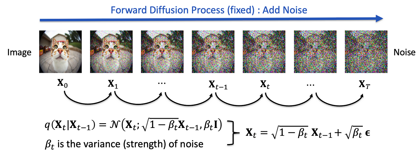Denoising Diffusion Probabilistic Models (DDPMs) are generative models that progressively add noise to data in a forward process, and then learn to invert this process to generate new data samples from noise. In the original DDPM (Ho et al., 2020), the forward diffusion is discrete, applying noise in \(N\) steps until data become (approximately) Gaussian. The reverse process is also defined discretely, denoising step by step. Recent perspectives (Song et al., 2021) have shown that we can view diffusion models in continuous time, describing them via SDEs. This text shows how the discrete forward process in DDPM converges to a continuous SDE when we let the number of steps \(N \to \infty\), and how the corresponding reverse SDE aligns with the DDPM reverse noising formula.

In the following sections, let's derivate the continous format of diffusion process by taking the timestep to limit 0.

3.1 Discrete Forward Process in DDPM

In the standard (discrete) DDPM, each forward step is:

\[ x_i \;=\; \sqrt{1 - \beta_i}\, x_{i-1} \;+\; \sqrt{\beta_i}\,\epsilon_i, \quad \epsilon_i \sim \mathcal{N}(0, I), \quad i=1,\dots,N. \]

• \(\beta_i \in [0,1]\) is the noise intensity at step \(i\).

• \(x_0\) is sampled from the real data distribution \(p_{\mathrm{data}}\).

• After \(N\) steps, \(x_N\) is (approximately) Gaussian. Often, \(\beta_i\) is chosen according to a schedule (e.g. linear, cosine) from a small value to a moderately larger one. Even if some \(\beta_i\) are not very small, we can view each step as adding Gaussian noise to the current sample.

3.2 Splitting Large Steps via Gaussian Additivity

A key observation is that a single “large step” of Gaussian noise can be split into many smaller Gaussian increments without changing the final distribution . Formally, if

$$ x_{i} \;=\; \sqrt{1-\beta_i}\,x_{i-1} \;+\; \sqrt{\beta_i}\,\epsilon_i, $$ we can represent \(\epsilon_i\) as the sum of \(M\) smaller Gaussians of variance \(\beta_i/M\). In other words, we can rewrite that same update with \(M\) micro-steps, each of which has variance \(\beta_i/M\). Because Gaussians are closed under convolution, \(M\) small steps or \(1\) big step produce the same marginal distribution for \(x_i\). When \(M \to \infty\), each micro-step becomes infinitesimally small. Hence, we can imagine the entire forward diffusion as a limit of infinitely many tiny Gaussian increments. This viewpoint paves the way to interpret the forward process as a stochastic differential equation.

In other point of view, since we want to get the continuous format by taking the \(N\) tends to infinity, corresponds the increment of \(x_t\) be infenitesimal, which also requires that \(\beta_i \to 0\). In this sense, we have enough confidence to assume that

\[\tag{1}\boxed{\beta_i = \beta(t_i)\Delta t},\quad \beta(x): X \to \mathbb{R^+}\]

3.3 From Discrete Updates to a Continuous SDE

3.3.1 Mapping Steps to Time

Let the total diffusion run over time \(t \in [0,1]\), with discrete steps \(t_i = i/N\). Denote \(\Delta t = 1/N\)

3.3.2 Taylor Expansion Argument

Consider one discrete step:

\[ x_{i}=\sqrt{1-\beta_i}\,x_{i-1} \;+\; \sqrt{\beta_i}\,\epsilon_i. \]

If \(\beta_i\) is small, we use a first-order expansion:

\[ \sqrt{1-\beta_i} \;\approx\; 1 \;-\; \tfrac12\,\beta_i. \]

Then

\[ x_i - x_{i-1}\;\approx\;-\tfrac12\,\beta_i\,x_{i-1}\;+\; \sqrt{\beta_i}\,\epsilon_i. \]

Suppose \(x_i = x_{t+\Delta t}\) and \(x_{i-1}= x_{t}\), Hence

\[ \begin{aligned} x_{t + \Delta t} - x_{t} &= -\frac{1}{2} \beta (t + \Delta t) \Delta t x_{t} + \sqrt{\beta(t+\Delta t)\Delta t}\epsilon_t\\ &\approx -\frac{1}{2} \beta (t ) \Delta t x_{t} + \sqrt{\beta(t)\Delta t}\epsilon_t \\ & = -\frac{1}{2} \beta (t ) x_{t} \Delta t + \sqrt{\beta(t)} \Delta t \epsilon_t \\ & = -\frac{1}{2} \beta (t ) x_{t} \Delta t + \sqrt{\beta(t)} \big(W(t+\Delta t)- W(t) \big)\\ & = -\frac{1}{2} \beta (t ) x_{t} \Delta t + \sqrt{\beta(t)} dW \end{aligned} \]

Note that

\[ W(t + \Delta t) - W(t) \sim \mathcal{N}(0, \Delta t). \]

Thus in the limit we get the SDE:

\[ d x = -\tfrac12\,\beta(t)\,x\,dt \;+\; \sqrt{\beta(t)}\,dw \]

This is often referred to as the Variance Preserving SDE (VP-SDE) in the score-based literature.

3.3.3 Splitting Steps Argument

Alternatively, if \(\beta_i\) is not initially small, we can split each “big step” into \(M\) micro-steps of size \(\beta_i/M\). If we then let \(N \to \infty\) and \(M \to \infty\), so that \(\beta_i/M \to 0\), the entire chain of \(N\times M\) micro-steps again converges to the same SDE. Both methods lead to the conclusion:

\[ \boxed{ \text{Forward SDE: } dx = -\tfrac12\,\beta(t)\,x\,dt \;+\; \sqrt{\beta(t)}\,dw. } \]

3.3.4 The Reverse SDE

Given a forward SDE of the form:

\[ dx = f(x,t)\,dt \;+\; g(t)\,dw, \]

the corresponding reverse-time SDE is derived by Anderson (1982) and extended by Song et al. (2021):

\[ d\tilde{x}=\bigl[f(\tilde{x}, t) \;-\; g(t)^2\,\nabla_{\tilde{x}}\log p_t(\tilde{x})\bigr]\;dt \;+\; g(t)\,d\tilde{w}, \]

where:

• \(\tilde{w}\) represents a Brownian motion in reverse time
• \(\nabla_{\tilde{x}}\log p_t(\tilde{x})\) is the score function (gradient of the log density) at time \(t\)

For our specific case where \(f(x,t) = -\frac{1}{2}\beta(t)x\) and \(g(t)=\sqrt{\beta(t)}\), the reverse SDE takes the form:

\[ d\tilde{x}(t)= - \bigl[\tfrac12\,\beta(t)\,\tilde{x}+\beta(t)\,\nabla_{\tilde{x}}\log p_t(\tilde{x})\bigr]\;dt \;+\;\sqrt{\beta(t)}\,d\tilde{w}. \]

3.3.5 Consistency with DDPM’s Reverse

Here we can derivate the reserve formula from the DDPM reverse discrete steps by taking into infinitesimal timestep, which should be matched with the above formula which derivated from FPE.

Review the reserve step in DDPM

\[\tag{5}\boxed{ x_{t-1} = \frac{1}{\sqrt{1-\beta_t}}\left(x_t - \frac{\beta_t}{\sqrt{1-\bar{\alpha}_t}}\,\epsilon_\theta(x_t,t)\right) + \sqrt{\tilde{\beta}_t}\,z,\quad z\sim\mathcal{N}(0,I)} \]

Recall that in the DDPM reverse process the update (when the network predicts the noise \(\epsilon_\theta\)) is given by

\[ x_{t-1} = \frac{1}{\sqrt{1-\beta_t}}\left(x_t - \frac{\beta_t}{\sqrt{1-\bar{\alpha}_t}}\,\epsilon_\theta(x_t,t)\right) + \sqrt{\tilde{\beta}_t}\,z,\quad z\sim \mathcal{N}(0,I), \]

with $$ \bar{\alpha}t = \prod}^t (1-\beta_s),\qquad \tilde{\betat = \frac{1-\bar{\alpha}\,\beta_t. $$}}{1-\bar{\alpha}_t

When the number of steps is large, one may view each update as occurring over a small time interval. In what follows we will reparameterize the discrete index in terms of a small time increment.

Suppose that in the original (forward) time variable \(t\) we write the update from \(t\) to \(t-\Delta t\) as

\[ x(t-\Delta t) = \frac{1}{\sqrt{1-\beta(t)\,\Delta t}}\left(x(t) - \frac{\beta(t)\,\Delta t}{\sqrt{1-\bar{\alpha}(t)}}\,\epsilon_\theta(x(t),t)\right) + \sqrt{\tilde{\beta}(t)\,\Delta t}\,z. \]

For a small time interval, we assume the noise variance scales as \(\beta(t)\,\Delta t\). Similarly, \(\tilde{\beta}(t)\,\Delta t\) represents the variance used in the reverse update. Note that in the continuous limit, we typically find that \(\tilde{\beta}(t)\) converges to \(\beta(t)\).

Expanding to first order in \(\Delta t\) gives

\[ \begin{aligned} x(t-\Delta t) &\approx \Bigl(1+\tfrac{1}{2}\beta(t)\Delta t\Bigr)\left(x(t) - \frac{\beta(t)\Delta t}{\sqrt{1-\bar{\alpha}(t)}}\,\epsilon_\theta(x(t),t)\right) + \sqrt{\tilde{\beta}(t)\Delta t}\,z\\ &\approx x(t) - \frac{\beta(t)\,\Delta t}{\sqrt{1-\bar{\alpha}(t)}}\,\epsilon_\theta(x(t),t)+ \frac{1}{2}\beta(t)x(t)\,\Delta t+ \sqrt{\tilde{\beta}(t)\Delta t}\,z. \end{aligned} \]

That is, the increment in the original (forward) time is

\[-\Delta x = x(t-\Delta t)-x(t) = \left[\frac{1}{2}\beta(t)x(t)-\frac{\beta(t)}{\sqrt{1-\bar{\alpha}(t)}}\,\epsilon_\theta(x(t),t)\right]\Delta t + \sqrt{\tilde{\beta}(t)\,\Delta t}\,z. \]

In the continuous limit, \(\sqrt{\Delta t}\,z\) becomes the differential \(dW\) of a standard Wiener process.

\[ \text{d} x =- \left[\frac{1}{2}\beta(t)\,x(t) -\frac{\beta(t)}{\sqrt{1-\bar{\alpha}(t)}}\,\epsilon_\theta\Bigl(x(t),\,t)\Bigr) \right]dt - \sqrt{\beta(t))}\,dW. \]

To complete our analysis of the reverse process, let's introduce a time change:

Let \(\tau = T - t\) and \(\tilde{x}(\tau) = x(T-\tau)\)

Under this transformation:

• \(d\tau = -dt\) (time reversal)
• \(d\tilde{x} = -dx\) (process reversal)

This leads to:

\[ \text{d} \tilde{x} =- \left[\frac{1}{2}\beta(T-\tau)\,\tilde{x}(\tau) -\frac{\beta(T-\tau)}{\sqrt{1-\bar{\alpha}(T-\tau)}}\,\epsilon_\theta\Bigl(\tilde{x}(\tau),\,T-\tau\Bigr) \right]\tau + \sqrt{\beta(T-\tau)}\,dW. \]

This derivation shows how one may obtain a continuous-time (SDE) formulation of the DDPM reverse process with an explicit reversed time mapping.

Recall the formula from the reverse‐time dynamics,

\[ dx = \Bigl[-\frac{1}{2}\beta(t)x - \beta(t)\,\nabla_x\log p_t(x)\Bigr]dt + \sqrt{\beta(t)}\,d\bar{w}. \]

Use the estimator of the gradient from learning

\[ \nabla_x\log p_t(x) \approx -\frac{1}{\sqrt{1-\bar{\alpha}(t)}}\,\epsilon_\theta(x,t), \]

We got

\[ dx = \left[-\frac{1}{2}\beta(t)x + \frac{\beta(t)}{\sqrt{1-\bar{\alpha}(t)}}\,\epsilon_\theta(x,t)\right]dt + \sqrt{\beta(t)}\,d\bar{w}. \]

4. Summary of Correspondence

In the continuous format, we name it as VP-SDE, refer score based SDE for more details.

	VP-SDE (Continuous)	DDPM (Discrete)
\(x_t\)	\(x_t = \sqrt{\alpha_t} x_0 + \sqrt{1 - \alpha_t} \epsilon\)	\(x_t = \sqrt{\bar{\alpha}_t} x_0 + \sqrt{1 - \bar{\alpha}_t} \epsilon\)
\(\alpha_t\)	\(\alpha_t = e^{-\int_0^t \beta(s) ds}\)	\(\bar{\alpha}_t = \prod_{s=1}^{t} (1 - \beta_s)\)
\(\beta_t\)	\(\beta_t^{\text{VP-SDE}} = d(-\log \alpha_t) / dt\)	\(\beta_t^{\text{DDPM}} \approx \beta_t^{\text{VP-SDE}} \Delta t\)
\(\sigma_t\)	\(\sigma_t =\sqrt{ 1 - \alpha_t}\)	\(\sigma_t =\sqrt{1 - \bar{\alpha}_t}\)
forward	\(dx = -\frac{1}{2} \beta(t) x dt + \sqrt{\beta(t)} dw\)	\(x_t = \sqrt{1 - \beta_t} x_{t-1} + \sqrt{\beta_t} \epsilon\)
backward	\(dx = -\frac{1}{2} \beta(t) \left( x + 2 s_\theta(x, t) \right) dt + \sqrt{\beta(t)} dw\)	\(x_{t-1} = \frac{1}{\sqrt{\alpha_t}} \left( x_t - \frac{1 - \alpha_t}{\sqrt{1 - \bar{\alpha}_t}} \epsilon_\theta(x_t, t) \right) + \sigma_t z\)
Flow ODE	\(dx = - \frac{1}{2} \beta(t)\left( x + s_\theta(x, t) \right) dt\)	Na
loss	\(\mathbb{E}_{t, x_0, \epsilon} \left[ \lambda_t \|s_\theta(x_t, t) + \frac{\epsilon_\theta(x,t)}{\sqrt{1-\alpha_t}} \|^2 \right] \)	\(\mathbb{E}_{t,x_0,\epsilon} \left[\| \epsilon_\theta(x,t) - \epsilon\|^2\right] \)
score function	\(-\frac{\epsilon}{\sqrt{1-\alpha_t}}\)
Reverse Sampling	\(x_{t-1} =x_{t} +\frac{1}{2} \beta(t) \left( x + 2 s_\theta(x, t) \right) dt - \sqrt{\beta(t)} dw\) or \(x_{t-1} =x_{t} +\frac{1}{2} \beta(t) \left( x + s_\theta(x, t) \right) dt\)	\(x_{t-1} = \frac{1}{\sqrt{\alpha_t}} \left( x_t - \frac{1 - \alpha_t}{\sqrt{1 - \bar{\alpha}_t}} \epsilon_\theta(x_t, t) \right) + \sigma_t z\)

5. Network Output: Noise Prediction vs. Score

In practice, DDPM commonly trains a network to predict the added noise \(\epsilon\) rather than directly predicting \(\nabla_x \log p(x_t)\) for better stability or convergence rage. However, there is a simple linear relation between \(\epsilon\) and the score. Therefore:

1. Predicting noise and predicting the score are equivalent in mathematical terms.

2. Score-based SDE models often produce \(\mathbf{s}_\theta(x,t) \approx \nabla_x \log p_t(x)\).

3. DDPM-like models produce \(\epsilon_\theta(x_t,t)\), from which the score can be derived.

Either way, we get a functional approximation to the same “denoising direction” that enables the reverse-time generative process.

Extenstion of the prediction types of diffusion model

Diffusion Target	Definition	Formula	Loss Function	Pros	Common Use Cases
\( \epsilon \)-Prediction (Noise Prediction)	Predicts the added noise.	\( \epsilon_\theta(x_t, t) \approx \epsilon \)	\( \mathbb{E} [ \| \epsilon - \epsilon_\theta(x_t, t) \|^2 ] \)	Standard DDPM target, works well in pixel space.	Classical DDPMs (e.g., OpenAI DDPM, ADM)
\( x_0 \)-Prediction (Data Prediction)	Predicts the clean image directly.	\( x_{0_\theta}(x_t, t) \approx x_0 \)	\( \mathbb{E} [ \| x_0 - x_{0_\theta}(x_t, t) \|^2 ] \)	Directly generates the final image.	Consistency Models, improved diffusion models
\( v \)-Prediction (Velocity Prediction)	Predicts a combination of noise and clean data.	\( v_\theta(x_t, t) = \alpha_t \epsilon - \sigma_t x_0 \)	\( \mathbb{E} [ \| v - v_\theta(x_t, t) \|^2 ] \)	More stable training, better for latent diffusion.	Stable Diffusion, Latent Diffusion Models
\( \Sigma \)-Prediction (Variance Prediction)	Predicts the variance of the noise.	\(p_\theta(x_{t-1} \| x_t) = \mathcal{N}(\mu_\theta, \Sigma_\theta)\)	\( \mathbb{E} [ \| \epsilon - \epsilon_\theta \|^2 + w(t) \cdot \text{KL}(\Sigma_\theta) ] \)	Better uncertainty estimation, prevents variance explosion.	Class-conditional DDPMs (ADM), Stable Diffusion
\( s \)-Prediction (Score Function Prediction)	Predicts the score function instead of noise.	\( s_\theta(x_t, t) = -\nabla_{x_t} \log p_t(x_t) \)	\( \mathbb{E} [ \| s_\theta - \nabla_{x_t} \log p_t(x_t) \|^2 ] \)	Works well in continuous-time diffusion models.	Score-Based Models (SGM), Continuous-Time Diffusion Models
EBM-Prediction (Energy-Based Model)	Learns an energy function.	\( \frac{\partial x}{\partial t} = -\nabla_x E_\theta(x, t) + \sigma \xi_t \)	N/A (Energy-Based Loss)	Unifies score-based and energy-based models.	Diffusion-EBMs

Key Takeaways

• Most standard diffusion models use \( \epsilon \)-prediction.
• \( v \)-prediction improves stability and is common in latent diffusion.
• \( \Sigma \)-prediction adds variance modeling for better flexibility.
• Score-based prediction is used in continuous-time models.
• EBMs provide an alternative energy-based formulation.

6. Appendix

6.1 What is the Fokker–Planck Equation?

Put simply, the Fokker–Planck equation describes how the probability density function (PDF) of a stochastic (random) process evolves over time. More formally, if we let \(p(x,t)\) be the probability density of finding the system in state \(x\) at time \(t\), the Fokker–Planck equation reads:

\[ \frac{\partial p(x,t)}{\partial t} = \left\lbrace -\frac{\partial}{\partial x} \left[ \mu(x)p(x,t)\right] + \frac{1}{2}\,\frac{\partial^2}{\partial x^2}(\,D(x)\,p(x,t))\right\rbrace \]

where

• \(\mu(x)\) represents the deterministic drift or “drift velocity”. It reflects the average effect of an external force acting on the system.

• \(D(x)\) represents the diffusion (random fluctuations) at state \(x\).

For simplicity, we often see the equation in the case of constant diffusion \(D\) and constant drift \(v\): $$ \frac{\partial p(x,t)}{\partial t} = -v\,\frac{\partial p(x,t)}{\partial x} + \frac{D}{2}\,\frac{\partial^2 p(x,t)}{\partial x^2}. $$

This partial differential equation tells us how the probability density changes because of both deterministic drift (\(v\)) and random diffusion (\(D\)).

---

6.2 When Does the Probability Follow the Fokker–Planck Equation?

The Fokker–Planck equation is typically valid under these conditions:

1. Continuous Markov processes in one dimension (or higher).

2. The process must be Markovian: the future depends only on the present state, not on the history.

3. Stochastic differential equations (SDEs) of the form

   \[ dX_t = \mu(X_t)\,dt + \sqrt{D(X_t)}\,dW_t, \]
   • where \(W_t\) is a standard Brownian motion (Wiener process).

4. Small, Gaussian-like noise.

5. The derivation of the Fokker–Planck relies on the assumption that increments of noise are small over short intervals (leading to the second-order derivative term in the FP equation).

6. No long-range jumps (no Lévy flights).

7. If jumps or large discontinuous moves exist, then we would use generalized kinetic equations (like fractional Fokker–Planck or Master equations) rather than the classical FP equation. In essence, if your system follows an Itô-type (or Stratonovich-type) SDE with drift \(\mu\) and diffusion coefficient \(D\), then the probability density of where that system might be at time \(t\) will satisfy the Fokker–Planck equation.

6.3 Intuitive Interpretation of Drift and Diffusion in the Fokker–Planck Equation

The Fokker–Planck equation is a powerful tool for describing how probability densities evolve over time. In many fields—such as physics, biology, and finance—it is used to capture the interplay between deterministic forces and random fluctuations. This blog post provides an intuitive explanation of the two key components: drift and diffusion .

6.3.1 Drift: The Deterministic Push

In the one-dimensional Fokker–Planck equation, the drift term is commonly written as:

\[ -\frac{\partial}{\partial x}\Big[A(x)P(x,t)\Big] \]

Here,

• \(A(x)\) represents the deterministic drift or “drift velocity”. It reflects the average effect of an external force acting on the system.

• \(P(x,t)\) is the probability density at position \(x\) and time \(t\).

• The product The product \(A(x)P(x,t)\) represents the probability flux resulting from the deterministic motion.

Imagine particles moving under the influence of an external force:

• Probability Flow: The term \(A(x)P(x,t)\) can be thought of as the flow of particles moving with velocity \(A(x)\). This is similar to how a group of people might move along a corridor when prompted by a guiding signal.

• Divergence and Local Density Change: The spatial derivative \(\frac{\partial}{\partial x}[A(x)P(x,t)]\) measures how the flow changes along the \(x\)-direction (its divergence).

• If the divergence is positive at a point, more particles are leaving that region than entering it. Because of the negative sign in the equation, this results in a decrease in the probability density (\(\frac{\partial P}{\partial t} < 0\)).

• Conversely, if the divergence is negative , particles are converging at that point, leading to an increase in the local density (\(\frac{\partial P}{\partial t} > 0\)).

This formulation captures how deterministic forces cause a net flow of probability, thereby modifying the local density.

6.3.2 Diffusion: The Smoothing Effect of Random Perturbations

The diffusion term in the Fokker–Planck equation is typically expressed as: $$ \frac{1}{2}\frac{\partial^2}{\partial x^2}\Big[B(x)P(x,t)\Big] $$

Here,

• \(B(x)\) is the diffusion coefficient, indicating the strength of random fluctuations.

• The second derivative \(\frac{\partial^2}{\partial x^2}\) reflects the curvature of the probability density, indicating how "peaked" or "spread out" the distribution is locally.

Diffusion describes how random perturbations work to smooth out irregularities in the probability distribution:

• High-Density Regions (Peaks): At locations where \(P(x,t)\) forms a peak, the distribution is concave down (negative curvature). The diffusion term acts to reduce the density at these peaks, causing the probability to spread out.

• Low-Density Regions (Valleys): In contrast, in regions where the density is low and the distribution is convex (positive curvature), diffusion causes the density to increase by “filling in” these valleys with probability from neighboring regions.

This effect is analogous to a drop of ink spreading on paper: the concentrated ink in the center disperses outward, leading to a more uniform concentration over time. Diffusion thus does not simply lower the density everywhere; rather, it redistributes it, diminishing local extremes to create a smoother overall profile.

---

6.3.2.1 Drift and Diffusion: Combined Evolution of the Probability Density

In the Fokker–Planck equation, drift and diffusion work together to dictate how the probability density evolves:

• Drift accounts for the systematic, directional movement driven by deterministic forces. It creates flows that can either concentrate or deplete the density depending on the spatial gradient (divergence) of the flux.

• Diffusion represents the effect of random fluctuations, working to smooth out the probability distribution. It reduces sharp peaks and fills in dips, leading to a more even spread of the density.

Together, these processes explain how the overall distribution changes over time, even if the motion of individual particles is unpredictable. By considering both the directional push of drift and the smoothing influence of diffusion, the Fokker–Planck equation provides a comprehensive framework for understanding the evolution of complex systems under uncertainty.

In the Fokker–Planck equation, drift and diffusion work together to dictate how the probability density evolves:

• Drift accounts for the systematic, directional movement driven by deterministic forces. It creates flows that can either concentrate or deplete the density depending on the spatial gradient (divergence) of the flux.

• Diffusion represents the effect of random fluctuations, working to smooth out the probability distribution. It reduces sharp peaks and fills in dips, leading to a more even spread of the density.

Together, these processes explain how the overall distribution changes over time, even if the motion of individual particles is unpredictable. By considering both the directional push of drift and the smoothing influence of diffusion, the Fokker–Planck equation provides a comprehensive framework for understanding the evolution of complex systems under uncertainty.

💬 Comments Share your thoughts!