Scalable Diffusion Models with Transformers (DiT)¶

Year: March 2023
Authors:
William Peebles
- DiT model (UC Berkeley)
- SORA project (OpenAI)
Saining Xie
- DiT model (New York University)
- ResNeXt
- Cambrian-1 with Yann LeCun
Main Contributions:
Replaced the U-Net backbone with transformers
Analyzed scalability properties
Repository: https://github.com/facebookresearch/DiT/tree/main

1. Diffusion Transformer Design¶

The transformer diffusion is also trained with the latent diffusion model. Thus, the transformer diffusion is designed on the latent space.

1.1 Patchify¶

Converts spatial input into a sequence of \(T\) tokens.
Suppose the input size is [64, 64, 4], \(p=16\). For each \(16\times16\) square, we flatten it into a single token with a linear embedding layer. In total, we obtain \(64\times 64 / (p^2) = 16\) tokens. The output shape should be [16, d].
In the design, the patch size \(p\) is regarded as a parameter.

We can use conv2d to perform patchification, followed by flattening and transposing to reshape the output.

import torch
import torch.nn as nn
# Define the patch size
patch_size = 16
# Create a convolutional layer to extract patches
# The number of output channels (embedding_dim) is a hyperparameter
embedding_dim = 768  # Example embedding dimension
patchify = nn.Conv2d(
    in_channels=4,       # Number of input channels
    out_channels=embedding_dim,  # Embedding dimension
    kernel_size=patch_size,      # Size of each patch
    stride=patch_size            # Stride to ensure non-overlapping patches
)
# Example input tensor with shape (batch_size, channels, height, width)
batch_size = 8  # Example batch size
input_tensor = torch.randn(batch_size, 4, 64, 64)  # Random input tensor
# Apply the patchify operation
patches = patchify(input_tensor)  # Shape: (batch_size, embedding_dim, 4, 4)
# Reshape patches to (batch_size, num_patches, embedding_dim)
# Here, num_patches = (64 / 16) * (64 / 16) = 4 * 4 = 16
patches = patches.flatten(2)  # Shape: (batch_size, embedding_dim, num_patches)
patches = patches.transpose(1, 2)  # Shape: (batch_size, num_patches, embedding_dim)
print(patches.shape)  # Output: torch.Size([batch_size, 16, 768])

1.2 Positional Encoding¶

Similar to the standard sine-cosine positional encoding, we can also use conv2d for positional encoding.

import torch
import torch.nn as nn
import math

class PositionalEncoding(nn.Module):
    def __init__(self, d_model, max_len=5000):
        super(PositionalEncoding, self).__init__()
        # Create a matrix of shape (max_len, d_model) to hold the positional encodings
        pe = torch.zeros(max_len, d_model)
        # Position indices (0, 1, 2, ..., max_len-1)
        position = torch.arange(0, max_len, dtype=torch.float).unsqueeze(1)
        # Compute the div_term for the exponential function
        div_term = torch.exp(torch.arange(0, d_model, 2).float() * (-math.log(10000.0) / d_model))
        # Apply sine to even indices in the array; 2i
        pe[:, 0::2] = torch.sin(position * div_term)
        # Apply cosine to odd indices in the array; 2i+1
        pe[:, 1::2] = torch.cos(position * div_term)
        # Add a batch dimension
        pe = pe.unsqueeze(0)
        # Register pe as a buffer to prevent it from being considered a model parameter
        self.register_buffer('pe', pe)

    def forward(self, x):
        # Add positional encoding to the input tensor
        x = x + self.pe[:, :x.size(1), :]
        return x

In transformer models, positional encoding is used to inject information about the position of tokens in a sequence, as the model itself doesn't inherently capture positional information. A common method is to use sinusoidal functions to generate these encodings. The formulas for sine and cosine positional encodings are as follows:

For a given position \( \text{pos} \) and embedding dimension \( i \):

When \( i \) is even:

\[ \text{PE}(\text{pos}, i) = \sin\left(\frac{\text{pos}}{10000^{\frac{i}{d_{\text{model}}}}}\right) \]

When \( i \) is odd:

\[ \text{PE}(\text{pos}, i) = \cos\left(\frac{\text{pos}}{10000^{\frac{i}{d_{\text{model}}}}}\right) \]

Here, \( d_{\text{model}} \) represents the dimensionality of the model's embeddings. These functions use different frequencies to encode each dimension, allowing the model to distinguish between different positions in the sequence. This approach was introduced in the "Attention Is All You Need" paper.

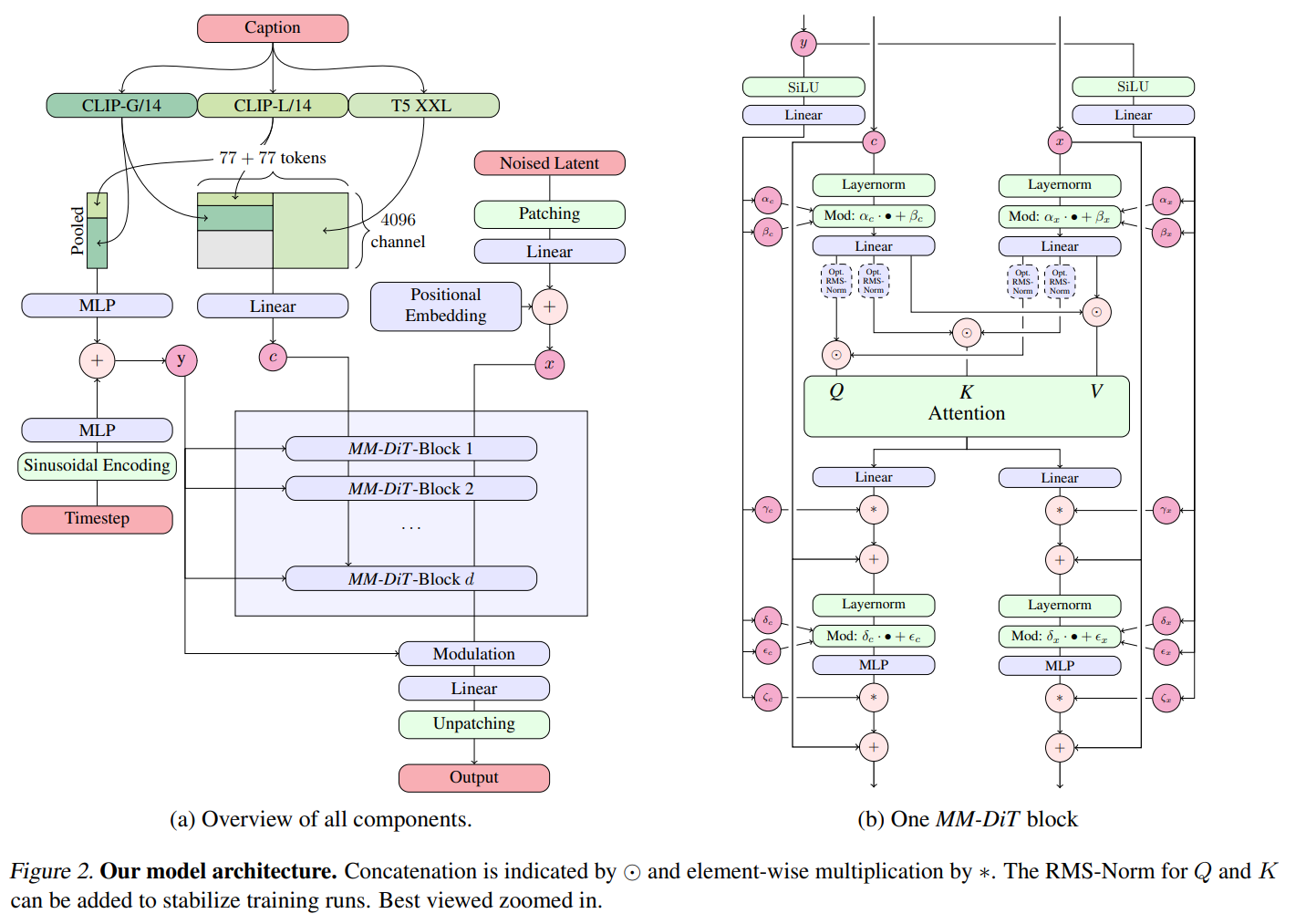
2. DiT Block Design¶

The core challenge is to design how to incorporate conditional information such as:

Timestep \(t\)
Class label \(c\)
Guided text
Guided spatial information such as depth, etc.

To implement this, the paper designs four different blocks to accept the conditions.

2.1 In-context Conditioning¶

Similar to the cls token in ViT, treat the embeddings of \(t\) and \(c\) as two additional tokens in the input sequence:

\[ [e_t, e_c, \text{patch}_1, \text{patch}_2, ..., \text{patch}_N] \]

Then the input sequence is passed through a transformer encoder to extract context information.

2.2 Cross Attention Block¶

Similar to the Latent Diffusion latent diffusion hands-on

The \(t\) and \(c\) are concatenated as a length-two sequence and act as \(K\) and \(V\) in the cross-attention block, as shown in the above picture.

2.3 Adaptive Layer Norm (adaLN)¶

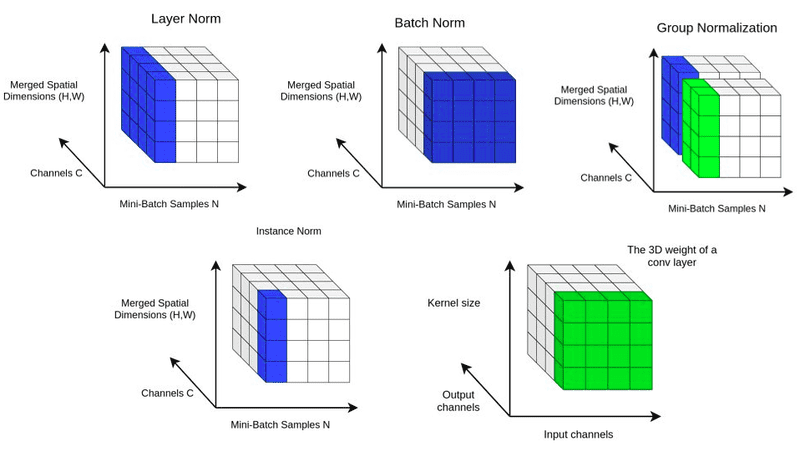
Borrowing ideas from StyleGAN's AdaIN, here is a comparison of Adaptive Layer Normalization (adaLN) in DiT and Adaptive Instance Normalization (AdaIN) in StyleGAN in tabular format:

Feature	adaLN (DiT)	AdaIN (StyleGAN)
Purpose	Modulates transformer layers based on conditioning input (e.g., class labels, text embeddings).	Transfers style by aligning content feature statistics to match style feature statistics.
Normalization Scope	Normalizes across the entire layer (layer normalization).	Normalizes each feature channel independently per instance. (instance normalization)
Mathematical Formula	\( o_i = \gamma(y) \cdot \frac{x_i - \mu}{\sigma + \epsilon} + \beta(y) \)	\( o_i = \sigma(y) \cdot \frac{x_i - \mu(x)}{\sigma(x) + \epsilon} + \mu(y) \)
Parameter Modulation	\( \gamma \) and \( \beta \) are dynamically generated from a conditioning input \( y \).	\( \mu(y) \) and \( \sigma(y) \) are extracted from the style input \( y \).
Dependency	Learns conditioning through a neural network (e.g., MLP).	Uses statistics (mean & variance) directly from the style input.
Application	Used in transformer-based models like DiT to condition the model on auxiliary data (e.g., text, class labels).	Used in StyleGAN for style transfer and control of image synthesis.

Here adaLN_modulation predicts the parameters \(\alpha_1\), \(\alpha_2\), \(\beta_1\), \(\beta_2\), \(\gamma_1\), \(\gamma_2\).

The DiTBlock with Adaptive Layer Norm Zero (adaLN-Zero) can be mathematically represented by the following function:

\[ (S_{\text{MSA}}, \alpha_{\text{MSA}}, G_{\text{MSA}}, S_{\text{MLP}}, \alpha_{\text{MLP}}, G_{\text{MLP}}) = f_{\text{adaLN}}(C) \]

Self attention

\[ X' = X + G_{\text{MSA}} \cdot \text{MSA} \left( \alpha_{\text{MSA}} \cdot \frac{X - \mu_X}{\sigma_X + \epsilon} + S_{\text{MSA}} \right) \]

Feedforward (MLP) Update

\[ X'' = X' + G_{\text{MLP}} \cdot \text{MLP} \left( \alpha_{\text{MLP}} \cdot \frac{X' - \mu_{X'}}{\sigma_{X'} + \epsilon} + S_{\text{MLP}} \right) \]

2.4 adaLN Zero Initialization¶

Assuming that zero initialization for residual networks is beneficial, we add the parameter \(scale\) to control the effects of adaLN. Initially, we set all the parameters of linear layers to 0.

2.5 Overall Structure of DiT¶

  def forward(self, x, t, y):
        """
        Forward pass of DiT.
        x: (N, C, H, W) tensor of spatial inputs (images or latent representations of images)
        t: (N,) tensor of diffusion timesteps
        y: (N,) tensor of class labels
        """
        x = self.x_embedder(x) + self.pos_embed  # (N, T, D), where T = H * W / patch_size ** 2
        t = self.t_embedder(t)                   # (N, D)
        y = self.y_embedder(y, self.training)    # (N, D)
        c = t + y                                # (N, D)
        for block in self.blocks:
            x = block(x, c)                      # (N, T, D)
        x = self.final_layer(x, c)                # (N, T, patch_size ** 2 * out_channels)
        x = self.unpatchify(x)                   # (N, out_channels, H, W)
        return x