Flux.1

Code explain: https://zhuanlan.zhihu.com/p/741939590/ reading note: https://zhuanlan.zhihu.com/p/684068402?utm_source=chatgpt.com

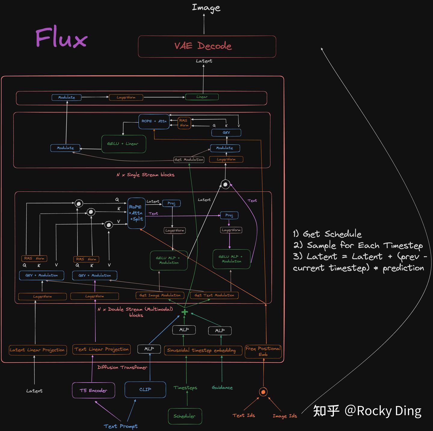
network structure

Code study¶

Next, let's study the code of flux.1 in details. Since the Flux only provided the inference code, we did not know how the model is trained. Let's just check how the model is sampled and try to guess how the model is trained.

We start with the sampling methods

1. Sampling¶

The flux sampling accept the following parameters:

    def generate_image(
        self,
        width,
        height,
        num_steps,
        guidance,
        seed,
        prompt,
        init_image=None,
        image2image_strength=0.0,
        add_sampling_metadata=True,

here $\text{width}$ and $\text{height}$ are the dimensions of the output image, $\text{num\_steps}$ is the number of denoising steps, $\text{guidance}$ is the guidance scale, $\text{seed}$ is the random seed, $\text{prompt}$ is the text prompt, $\text{init\_image}$ is the optional initial image, $\text{image2image\_strength}$ is the strength of the image-to-image guidance, and $\text{add\_sampling\_metadata}$ is a boolean indicating whether to add sampling metadata.

@dataclass
class SamplingOptions:
    prompt: str
    width: int
    height: int
    num_steps: int
    guidance: float
    seed: int | None

2. time scheduling¶

2.1 `time_shift` 函数¶

def time_shift(mu: float, sigma: float, t: Tensor):
    return math.exp(mu) / (math.exp(mu) + (1 / t - 1) ** sigma)

数学表达式： $$ \text{time_shift}(\mu, \sigma, t) = \frac{e^\mu}{e\mu + \left(\frac{1}{t} - 1\right)^\sigma} $$

参数说明： • $\mu$：控制函数曲线的中心位置。 • $\sigma$：控制函数曲线的陡峭程度。 • $t$：输入的时间张量，取值范围为 $[0, 1]$。

功能： • 对输入的时间 $t$ 进行非线性变换，使其在 $[0, 1]$ 区间内重新分布。 • 当 $\mu$ 增大时，函数曲线向右偏移；当 $\sigma$ 增大时，函数曲线变得更陡峭。

2.2 `get_lin_function` 函数¶

def get_lin_function(
    x1: float = 256, y1: float = 0.5, x2: float = 4096, y2: float = 1.15
) -> Callable[[float], float]:
    m = (y2 - y1) / (x2 - x1)
    b = y1 - m * x1
    return lambda x: m * x + b

数学表达式： $$ \text{get_lin_function}(x_1, y_1, x_2, y_2) = f(x) = m \cdot x + b $$ 其中： $$ m = \frac{y_2 - y_1}{x_2 - x_1}, \quad b = y_1 - m \cdot x_1 $$

参数说明： • $x_1, y_1$：直线上的第一个点。 • $x_2, y_2$：直线上的第二个点。 • $x$：输入的自变量。

功能： • 根据两点 $(x_1, y_1)$ 和 $(x_2, y_2)$ 计算直线的斜率和截距，返回一个线性函数 $f(x) = m \cdot x + b$。也就是根据分辨率计算时间步长的调整参数。256 对应的 $\mu$ 值为 0.5，4096 对应的 $\mu$ 值为 1.15。

2.3 `get_schedule` 函数¶

def get_schedule(
    num_steps: int,
    image_seq_len: int,
    base_shift: float = 0.5,
    max_shift: float = 1.15,
    shift: bool = True,
) -> list[float]:
    # extra step for zero
    timesteps = torch.linspace(1, 0, num_steps + 1)

    # shifting the schedule to favor high timesteps for higher signal images
    if shift:
        # estimate mu based on linear estimation between two points
        mu = get_lin_function(y1=base_shift, y2=max_shift)(image_seq_len)
        timesteps = time_shift(mu, 1.0, timesteps)

    return timesteps.tolist()

数学表达式： 1. 生成时间步长： $$ \text{timesteps} = \text{linspace}(1, 0, \text{num_steps} + 1) $$ 2. 如果需要调整时间步长： $$ \mu = f(\text{image_seq_len}), \quad \text{timesteps} = \text{time_shift}(\mu, 1.0, \text{timesteps}) $$ 其中 $f$ 是由 get_lin_function 生成的线性函数： $$ f(x) = m \cdot x + b, \quad m = \frac{\text{max_shift} - \text{base_shift}}{x_2 - x_1}, \quad b = \text{base_shift} - m \cdot x_1 $$

参数说明： • $\text{num\_steps}$：时间步长的数量。 • $\text{image\_seq\_len}$：图像序列的长度，用于计算 $\mu$。 • $\text{base\_shift}$：时间调整的基础值。 • $\text{max\_shift}$：时间调整的最大值。 • $\text{shift}$：是否对时间步长进行调整。

功能： 1. 生成从 1 到 0 的等间隔时间步长。 2. 如果需要调整时间步长： • 根据 $\text{image\_seq\_len}$ 计算 $\mu$。 • 使用 time_shift 函数对时间步长进行非线性变换。

2.4 整体逻辑¶

生成时间步长： $$ \text{timesteps} = {1, 1 - \Delta, 1 - 2\Delta, \dots, 0}, \quad \Delta = \frac{1}{\text{num_steps}} $$
计算 $\mu$： $$ \mu = f(\text{image_seq_len}), \quad f(x) = m \cdot x + b $$
调整时间步长： $$ \text{timesteps} = \left{ \frac{e^\mu}{e\mu + \left(\frac{1}{t} - 1\right)^\sigma} \mid t \in \text{timesteps} \right} $$ 调整后时间步长的效果

3. 图片和prompt预处理¶

```py3
def prepare(self, img: Tensor, prompt: str | list[str]) -> dict[str, Tensor]:
    ## process initial image and prompt
    bs, c, h, w = img.shape
    if bs == 1 and not isinstance(prompt, str):
        bs = len(prompt)
    img = rearrange(img, "b c (h ph) (w pw) -> b (h w) (c ph pw)", ph=2, pw=2)
    if img.shape[0] == 1 and bs > 1:
        img = repeat(img, "1 ... -> bs ...", bs=bs)
    img_ids = torch.zeros(h // 2, w // 2, 3)
    img_ids[..., 1] = img_ids[..., 1] + torch.arange(h // 2)[:, None]
    img_ids[..., 2] = img_ids[..., 2] + torch.arange(w // 2)[None, :]
    img_ids = repeat(img_ids, "h w c -> b (h w) c", b=bs)
    if isinstance(prompt, str):
        prompt = [prompt]
    txt = self.t5(prompt)
    if txt.shape[0] == 1 and bs > 1:
        txt = repeat(txt, "1 ... -> bs ...", bs=bs)
    txt_ids = torch.zeros(bs, txt.shape[1], 3)
    vec = self.clip(prompt)
    if vec.shape[0] == 1 and bs > 1:
        vec = repeat(vec, "1 ... -> bs ...", bs=bs)
    return {
        "img": img,
        "img_ids": img_ids.to(img.device),
        "txt": txt.to(img.device),
        "txt_ids": txt_ids.to(img.device),
        "vec": vec.to(img.device),
    }
```

不同于SD 3, 这里只用到两个text encoder, 一个是clip, 一个是t5,分别用于global的文本特征和局部的文本特征，也就是 'vec'和'txt',相对于SD 3,会更简洁。

同时这里增加了'img_ids'和'txt_ids',用来给图片和文本添加位置编码。其中'img_ids'是图片的坐标，'txt_ids'是文本的坐标，目前为0。

因为整张图片会被分成很多个$2\times 2$ 的小块，这个'img_ids'记录的就是每个小块的编号，从而让模型知道这个小块在图片中的位置。

4. 去噪步骤¶

```py3 title="Denoise"
  for t_curr, t_prev in zip(timesteps[:-1], timesteps[1:]):
        t = torch.full((img.shape[0],), t_curr, dtype=img.dtype, device=img.device)
        pred = self.model(
            img=torch.cat((img, img_cond), dim=-1) if img_cond is not None else img,
            img_ids=img_ids,
            txt=txt,
            txt_ids=txt_ids,
            y=y,
            timesteps=t,
            guidance=guidance,
        )
        img = img + (t_prev - t_curr) * pred
```

用数学公式表示就是：

\[ x_{t_{n-1} } = x_{t_{n}} + (t_{n} - t_{n-1}) \cdot f_\text{pred} \]

where $t_n,n=0,1,\ldots,N-1$ starts from 1 and ends at 0.

这是一个标准的Euler去噪步骤, 对应的ODE是

\[\frac{\mathrm{d} x}{\mathrm{d} t} = f_\text{pred}(x,t)\]

5. Flux Model¶

接下来我们看一下flux model 的网络结构，看它怎么处理图片以及condition的。它主要的结构包括 - guidance embedding & time embedding - positional encoding - double stream block - single stream block - output layer

1. Double Stream Block¶

1.1 1. 输入与参数定义¶

• 输入： • 图像特征：$ \mathbf{X}_{\text{img}} \in \mathbb{R}^{B \times L_{\text{img}} \times D} $ • 文本特征：$ \mathbf{X}_{\text{txt}} \in \mathbb{R}^{B \times L_{\text{txt}} \times D} $ • 调制向量：$ \mathbf{v} \in \mathbb{R}^{B \times d} $ • 位置编码：$ \mathbf{P} \in \mathbb{R}^{L \times d_p} $ • 参数生成（通过 img_mod 和 txt_mod）： • 图像调制参数： $$ (\mathbf{s}{\text{img}}^{(1)}, \mathbf{b}}}^{(1)}, g_{\text{img}}^{(1)}), \quad (\mathbf{s{\text{img}}^{(2)}, \mathbf{b}) $$ • 文本调制参数： $$ (\mathbf{s}}}^{(2)}, g_{\text{img}}^{(2)}) = \text{img_mod}(\mathbf{v{\text{txt}}^{(1)}, \mathbf{b}}}^{(1)}, g_{\text{txt}}^{(1)}), \quad (\mathbf{s{\text{txt}}^{(2)}, \mathbf{b}) $$}}^{(2)}, g_{\text{txt}}^{(2)}) = \text{txt_mod}(\mathbf{v

1.2 2. 图像分支处理¶

1.2.1 (a) 特征调制¶

• 归一化： $$ \mathbf{X}{\text{img}}^{(1)} = \text{Norm}_1^{\text{img}}(\mathbf{X}) $$ • }仿射变换： $$ \tilde{\mathbf{X}}{\text{img}}^{(1)} = \left(1 + \mathbf{s}}}^{(1)} \right) \odot \mathbf{X{\text{img}}^{(1)} + \mathbf{b} $$}}^{(1)

1.2.2 (b) 生成Q/K/V¶

• 线性投影： $$ \mathbf{Q}{\text{img}}, \mathbf{K}}}, \mathbf{V{\text{img}} = \text{split_heads}\left( \mathbf{W} \right) $$ 其中 }}^{qkv} \tilde{\mathbf{X}}_{\text{img}}^{(1)$ \mathbf{W}_{\text{img}}^{qkv} \in \mathbb{R}^{D \times 3HD} $，split_heads 将张量分割为多头形式。

1.2.3 (c) Q/K归一化¶

\[ \mathbf{Q}_{\text{img}}, \mathbf{K}_{\text{img}} = \text{Norm}_{\text{attn}}^{\text{img}}(\mathbf{Q}_{\text{img}}, \mathbf{K}_{\text{img}}) \]

1.3 3. 文本分支处理¶

1.3.1 (a) 特征调制¶

• 归一化： $$ \mathbf{X}{\text{txt}}^{(1)} = \text{Norm}_1^{\text{txt}}(\mathbf{X}) $$ • }仿射变换： $$ \tilde{\mathbf{X}}{\text{txt}}^{(1)} = \left(1 + \mathbf{s}}}^{(1)} \right) \odot \mathbf{X{\text{txt}}^{(1)} + \mathbf{b} $$}}^{(1)

1.3.2 (b) 生成Q/K/V¶

• 线性投影： $$ \mathbf{Q}{\text{txt}}, \mathbf{K}}}, \mathbf{V{\text{txt}} = \text{split_heads}\left( \mathbf{W} \right) $$}}^{qkv} \tilde{\mathbf{X}}_{\text{txt}}^{(1)

1.3.3 (c) Q/K归一化¶

\[ \mathbf{Q}_{\text{txt}}, \mathbf{K}_{\text{txt}} = \text{Norm}_{\text{attn}}^{\text{txt}}(\mathbf{Q}_{\text{txt}}, \mathbf{K}_{\text{txt}}) \]

1.4 4. 跨模态注意力¶

1.4.1 (a) 拼接Q/K/V¶

\[ \mathbf{Q} = [\mathbf{Q}_{\text{txt}}, \mathbf{Q}_{\text{img}}], \quad \mathbf{K} = [\mathbf{K}_{\text{txt}}, \mathbf{K}_{\text{img}}], \quad \mathbf{V} = [\mathbf{V}_{\text{txt}}, \mathbf{V}_{\text{img}}] \]

1.4.2 (b) 注意力计算¶

$$ \text{Attn}(\mathbf{Q}, \mathbf{K}, \mathbf{V}, \mathbf{P}) = \text{Softmax}\left( \frac{\mathbf{Q} \mathbf{K}^\top}{\sqrt{d}} + \phi(\mathbf{P}) \right) \mathbf{V} $$ 其中 $ \phi(\mathbf{P}) $ 为位置编码的映射函数。

1.4.3 (c) 分割注意力结果¶

\[ \mathbf{A}_{\text{txt}}, \mathbf{A}_{\text{img}} = \text{split}(\text{Attn}, [L_{\text{txt}}, L_{\text{img}}]) \]

1.5 5. 残差连接与输出¶

1.5.1 (a) 图像分支更新¶

• 注意力残差： $$ \mathbf{X}{\text{img}} \leftarrow \mathbf{X}}} + g_{\text{img}}^{(1)} \cdot \mathbf{W{\text{img}}^{\text{proj}} \mathbf{A} $$ • }MLP残差： $$ \mathbf{X}{\text{img}} \leftarrow \mathbf{X}}} + g_{\text{img}}^{(2)} \cdot \text{MLP{\text{img}} \left( \left(1 + \mathbf{s}}}^{(2)} \right) \odot \text{Norm2^{\text{img}}(\mathbf{X} \right) $$}}) + \mathbf{b}_{\text{img}}^{(2)

1.5.2 (b) 文本分支更新¶

• 注意力残差： $$ \mathbf{X}{\text{txt}} \leftarrow \mathbf{X}}} + g_{\text{txt}}^{(1)} \cdot \mathbf{W{\text{txt}}^{\text{proj}} \mathbf{A} $$ • }MLP残差： $$ \mathbf{X}{\text{txt}} \leftarrow \mathbf{X}}} + g_{\text{txt}}^{(2)} \cdot \text{MLP{\text{txt}} \left( \left(1 + \mathbf{s}}}^{(2)} \right) \odot \text{Norm2^{\text{txt}}(\mathbf{X} \right) $$}}) + \mathbf{b}_{\text{txt}}^{(2)

1.6 符号说明¶

• $ \odot $: 逐元素乘法（Hadamard积） • $ \text{Norm} $: 归一化操作（如LayerNorm或RMSNorm） • $ \text{MLP} $: 多层感知机（通常为线性层 + 激活函数 + 线性层） • $ \mathbf{W}^{qkv}, \mathbf{W}^{\text{proj}} $: 可学习的投影矩阵 • $ g $: 门控标量（控制残差分支的权重）

1.7 总结¶

该模块通过跨模态注意力融合图像与文本特征，利用动态调制参数（由向量 $\mathbf{v}$ 生成）对特征进行归一化和仿射变换，最终通过门控残差连接更新特征。数学公式完整描述了代码中的张量操作与信息流动。